This article is the first of a series on valuation adjustments, abbreviated to XVA. Here, we start with an introduction to the Counterparty Credit Risk (CCR) and CVA. In particular, we will see what these terms mean, how they arise, how they are computed and for which purpose, and what challenges they raise.

• Notation and abbreviations
• Counterparty Credit Risk
  • OTC derivatives
  • Counterparty credit risk (CCR)
  • Mitigants
    • Contract clauses
    • Central clearing
    • Close-out netting
    • Collateral
• CCR metrics and the CVA
  • Exposure metrics
    • EE: the expected exposure
    • PFE: the potential future exposure
  • CVA: the credit valuation adjustment
    • Incremental and marginal CVA
    • The CVA desk
    • Summary of CVA usage
    • Wrong Way Risk
• Challenges
  • Modelling challenge
  • Computational challenge
  • Continuous and rapid evolution
• References

Notation and abbreviations

Throughout this article, the following notation and abbreviations will be used:

• \(\beta(t)\): the money market account numéraire value at \(t\), defined by: \(\beta(t) = e^{\int_0^t r(u) du}\) where \(r\) is the short rate.
• \(V_i(t)\) : the market value or MtM of trade \(i\) at date \(t\).
• \(E(t)\) : the credit exposure at date \(t\).
• \(LGD\) : the loss given default.
• \(NDP(t)\) : the non-default probability between today and date \(t\).
• \(X^+\): the positive part of quantity \(X\), defined as: \(X^+= \max(X, 0)\).
• \(CCR\): the Counterparty Credit Risk.
• \(CVA\): the Credit Valuation Adjustment.
• \(MPOR\): the Margin Period Of Risk, the time interval from the last exchange of collateral and until the defaulting counterparty is closed out.

Counterparty Credit Risk

OTC derivatives

Financial derivatives are contracts to buy/sell an underlying security, or to make/receive payments whose value depends on an underlying security or index, at a time or times in the future that can range from weeks or months (e.g. FX forwards) to decades (e.g. interest rate swaps).

They are exchanged by financial institutions:

• banks and hedge funds;
• asset managers, pension funds and insurance companies;
• central banks, the IMF, the World Bank, etc.

but also by sovereigns, local authorities, non-financial corporations, etc.

Financial derivatives can serve many purposes, including:

• hedging or insurance, for example against a potential default using a credit default swap;
• investment, sometimes giving access to a market when the underlying is not directly tradeable (e.g. weather derivatives);
• but also for leverage, speculation, arbitrage, etc.

These contracts can be traded at an exchange, in this case they are called listed or exchange-traded, or bilateraly and in this case they are called over-the-counter or OTC derivatives

Evolution of the total outstanding notional of OTC derivatives

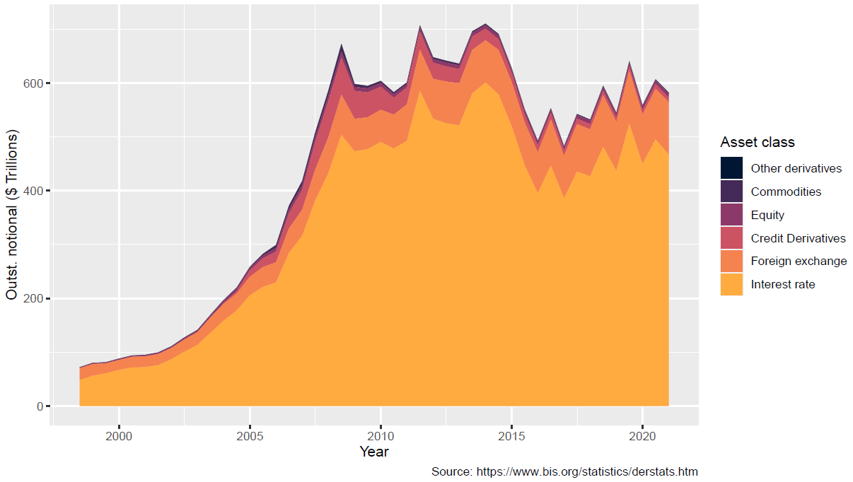
As no third party is involved in OTC derivatives, they can be flexible, allowing to match the exact need of the investor (e.g. tailor-made payoff) or the hedger (no basis risk). This flexibility has made them very successfull as shown by the rapid rise of their total outstanding notional during the 2000s, as illustrated in the above graph.

However, this comes at a cost of:

• less liquidity: in general, the more customized or sophisticated the derivative is, the less liquid it will be;
• more counterparty credit risk (CCR): the individual banks are less solid compared with the exchanges;
• they can also lead to systemic risk (e.g. through the G-SIBs).

Counterparty credit risk (CCR)

Counterparty credit risk (CCR) is the risk that the counterparty in a transaction could default before the final settlement of the transaction’s cash flows. In this case, an economic loss would occur if the transaction has a positive market value at the time of default.

This value is called the credit exposure (or in short, the exposure). For a date \(t\):

\[E(t) = V(t)^+\]

The drivers of the counterparty credit risk are :

• the market value of the positions with the counterparty, driven by underlying risk factors (e.g. interest and FX rates, equity prices, etc.);
• the counterparty’s default probability;
• and their correlation.

CCR is not as simple as lending risk because the future exposure is uncertain. For a loan, the exposure of the lender is simply the amount lent, while for an OTC derivative, the exposure will change with the market conditions. What’s more, as this market value can be positive or negative depending on the market conditions, CCR is bilateral whereas for simple loans only the lender assumes lending risk.

CCR is sometimes also called replacement risk or pre-settlement risk.

Mitigants

To reduce CCR, various mitigants are commonly used:

Contract clauses

These are clauses within each OTC contract that aim to reduce the CCR.

The first example are break clauses, which allow the contract to be terminated before its maturity by one or both parties. They can be mandatory, optional, or even contingent on some defined event such as a rating downgrade for example.

The second example are notional reset clauses, which reset the notional periodically to bring the contract’s market value to zero, thus resetting the CCR. This is typically the case for resetting cross currency swaps, also called marked-to-market cross currency swaps.

Central clearing

In 2009, the G20 leaders agreed to require mandatory central clearing for standardized derivatives. As of today, the main derivatives that are cleared are interest rate swaps and credit default swaps, but the coverage is increasing.

With central clearing, the CCP effectively becomes the counterparty of the buyer and seller, and centralizes the CCR by acting as intermediary.

This CCR concentration can be dangerous if the CCP fails. As a result, CCPs are highly regulated. To be approved, a CCP must put in place various mechanisms (e.g. margins, default fund, etc.) making it resilient and ensuring that the impact on the market will be as low as possible in the event of default.

The list of CCPs authorized to operate in the EU can be found here.

Close-out netting

Close-out netting is the process of combining positive and negative market values into a single net payable or receivable in the event of a default. It is governed by a master agreement such as the ISDA Master Agreement.

In the absence of this netting, the exposure of a set of contracts is simply the sum of exposures. In the presence of netting, the exposure of the netting set \(NS\) is lower than the sum of standalone exposures:

\[E^\text{(netting)}_{NS}(t) = \left(\sum_{i \in NS} V_i(t)\right)^+ \leq \sum_{i \in NS} V_i(t)^+\]

Netting agreements are signed between most banks, as well as some major non-financial institutions.

Collateral

To further mitigate CCR, financial institutions exchange collateral. The Credit Support Annex (CSA) of the master agreement specifies all its clauses such as:

• the types of contracts that are covered by the collateral exchange;
• the threshold amount below which no collateral is exchanged;
• the minimum transfer amount (MTA) aiming to decrease the operational cost;
• downgrade triggers ensuring more protection is required after a downgrade of the counterparty;
• eligible collateral types and currencies: cash, AAA bonds, etc.;
• the frequency of collateral exchange, etc.

Collateral agreements are signed between most banks, as well as some major non-financial institutions.

In the presence of collateral balance of \(C\), the exposure becomes:

\[E(t) = \left(V(t) - C(t) \right)^+\]

The collateral can be:

• segregated, meaning that it is held by a custodian and cannot be used.
• or it can be rehypothecated, that is used as collateral in another transaction, or lent, etc.

This will of course have an impact on whether the collateral can be recovered in the event of default, but let’s not get into these details here.

The collateral balance \(C(t)\) considered when computing the credit exposure at future date \(t\) is actually its value at \(t - MPOR\). This is because any collateral exchange with the defaulting counterparty is assumed to have stopped starting this date and until the close-out at \(t\). This period is usually around 2 weeks.

It is for this reason that the market value at \(t-MPOR\) is considered when computing \(C(t)\) in the next subsections.

There are two types of collateral.

Variation Margin

The first is variation margin and aims to track the variation of the aggregated market value.

The variation margin balance consists of the difference between the collateral received and posted. It is computed as the excess of positive (resp. negative) market value above (resp. below) the threshold + MTA. Denoting \(H\) the sum of the MTA and threshold amounts, and \(\bar{H}\) the same quantity for the institution from the counterparty’s point of view, that is:

\[C_\text{VM}(t)= \left( V(t − MPOR) − H \right)^+ - \left( V(t − MPOR) + \bar{H}\right)^−\]

The following graphs illustrate this for a trajectory of market value.

Variation margin computation: lagged MV

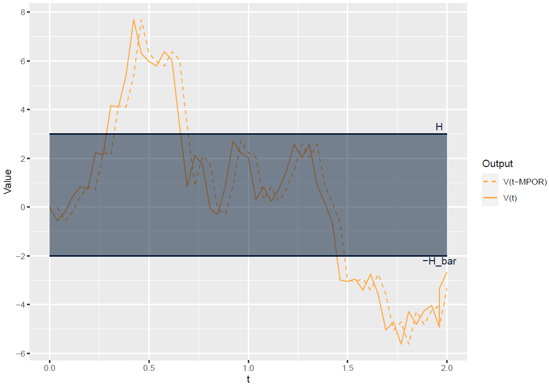
In the first graph, the market value \(V\) is lagged by the MPOR, then compared to \(H\) and \(-\bar{H}\) to get the variation margin (illustrated in the next graph). Any exposure in the blue area is accepted, and variation margin aims at remove any excess.

Variation margin computation: collateral balance and exposure

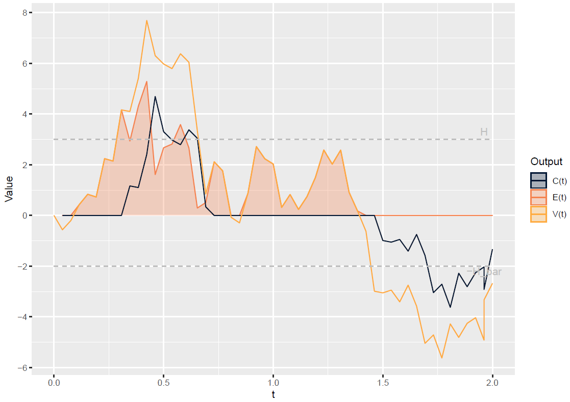
The second graph illustrates the resulting variation margin collateral balance \(C(t)\) and shows how it reduces the exposure \(E(t)\). Although it should in principle keep the exposure bellow \(H\), this is not always the case due to the MPOR.

Initial Margin

As no variation margin exchange takes place during the MPOR, the market value can diverge significantly from the collateral balance during this period, due to changing market conditions.

Initial margin and variation margin

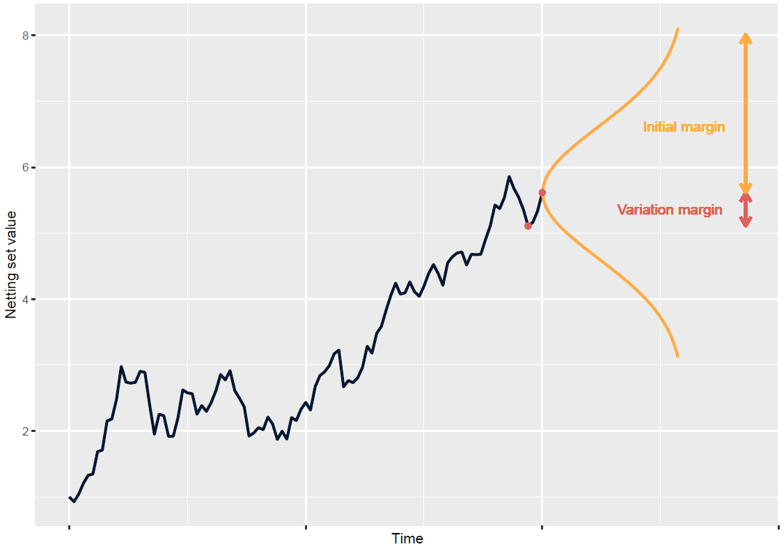
The initial margin aims to address this by covering losses due to market moves during the MPOR. It is usually computed as a quantile of market value variations over this period, with a confidence level \(\alpha\), for example \(99\%\):

\[\mathbb{P} \left[ \Delta V (t - MPOR, t) > C_\text{IM}^{(\alpha)}(t) \right] = 1 - \alpha\]

where \(\Delta V (t - MPOR, t)\) denotes the market value variation between \(t - MPOR\) and \(t\) coming only from market conditions, excluding any cash flows paid or received during this time interval.

Cleared trades are subject to initial margin, computed by CCPs using proprietary methodologies, involving historical expected shortfall at a high confidence level with zero threshold.

For uncleared bilateral trades, initial margin was introduced in 2011 by the G20 leaders, which was translated into a set of requirements by BCBS and IOSCO¹. It is posted by both parties, and computed according to the ISDA SIMM™ methodology² as a parametric value at risk with a threshold of USD 50M.

Initial margin turns the CCR into a funding cost for the initial margin to post, thus highly reducing the CVA, and introducing a funding cost of the posted initial margin captured by the MVA (margin valuation adjustment).

CCR metrics and the CVA

The computation of CCR metrics or of the CVA, relies on Monte-Carlo simulation. The computation is done in 4 steps:

1. Calibration: the model parameters are determined.
2. Diffusion: risk factors are simulated at future dates and for each Monte-Carlo scenario.
3. Pricing: the market values of the trades are computed.
4. Aggregation: the market values are aggregated to get the exposure metrics and/or CVA value.

For CCR metrics such as the PFE used for limits control, the Monte-Carlo simulation is done under the real-world measure, meaning that the diffusion models are calibrated on historical time series.

For CVA computations, it is done under the risk-neutral measure, meaning that the calibration is done on the financial instruments that will be used for hedging.

Exposure metrics

Many metrics exist to measure the credit exposure, we will give here the most common examples:

EE: the expected exposure

It is the expectation of the exposure. Usually a profile is computed, consisting in the EE values for various dates in the future \((t_i)_{1\leq i \leq n}\):

\[EE(t_i) = \mathbb{E} \left[ E(t_i) \right], \quad 1 \leq i \leq n\]

Most often, the EE is discounted to today:

\[EE(t_i) = \mathbb{E} \left[ \frac{E(t_i)}{\beta(t_i)} \right], \quad 1 \leq i \leq n\]

It is used as an intermediary computation step to get the CVA as we will see next, or to get other metrics used in regulatory computations, most notably the Effective Expected Positive Exposure (EEPE) defined as follows:

\[\begin{aligned} EEPE(t_n) &= \frac{1}{n} \sum_{i=1}^n EEE(t_i) (t_i - t_{i-1}) \\ EEE(t_i) &= \max \left(EE(t_i), EEE(t_{i-1}) \right), \quad 1 \leq i \leq n \end{aligned}\]

PFE: the potential future exposure

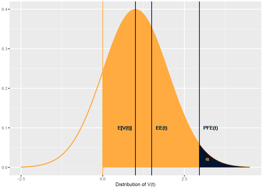
The PFE is the maximum future exposure at a specified future date with a given level of confidence \(\alpha\), usually 95% or 99%. In other words, it is a quantile of the exposure.

Just like the EE, what is usually computed is a PFE profile:

\[\mathbb{P}\left[ E(t_i) > PFE^{(\alpha)}(t_i) \right] = 1 - \alpha, \quad 1 \leq i \leq n\]

Unlike the value at risk, which considers the least favorable cases in terms of market value evolution (left hand side of the distribution), the PFE is concerned with the most favorable cases where we stand to lose the most in the event of counterparty default (right hand side of the distribution).

Expected market value, EE and PFE

The PFE is used for limits control. For a new trade to be authorised, the new PFE profile, including the candidate trade, has to be bellow the limits profile that is set by the risk department for this counterparty.

CVA: the credit valuation adjustment

The CVA is the expected loss arising from a counterparty default in the future. Denoting \(T\) the maturity of the longest trade with a given counterparty, and \(\tau\) the time of its default, that is:

\[\begin{aligned} CVA &= \mathbb{E}\left[ 1_{\{\tau \leq T\}} \times LGD \times \frac{E(\tau)}{\beta(\tau)}\right]\\ &= \int_0^T \mathbb{E}\left[ LGD \times \frac{E(t)}{\beta(t)} | \tau = t \right] dP(t) \end{aligned}\]

The formula is usually simplified by assuming a constant LGD and independence between the default and the exposure. Furthermore, the time integral is discretized on sample dates:

\[0 = t_0 < t_1 < \dots < t_n = T\]

leading to an expression of the form:

\[CVA = LGD \sum_{i=1}^n EE(t_i) \left(NDP(t_{i-1}) - NDP(t_i) \right)\]

The CVA reduces the base value of the portfolio of transactions with the counterparty, to take into account the possibility of its default:

\[V_\text{CCR} = V_\text{no CCR} - CVA\]

It is a value adjustment and is destined to be hedged, all expectations above is taken under the risk-neutral measure.

Incremental and marginal CVA

The CVA value above concerns the whole portfolio of trades with the counterparty. How is this amount charged or passed down to the counteparty?

During the trading day, the impact of each candidate trade (denoted \(j\) bellow) on the CVA position, called its incremental CVA is computed, and charged to the counterpart:

\[V_\text{CCR}(j) = V_\text{no CCR}(j) - {CVA}_\text{incremental}(j)\\ {CVA}_\text{incremental}(j) = {CVA}(\text{with }j) − {CVA}(\text{without }j)\]

This way, at the end of the day, the equality of the previous section is recovered, as the total CVA is the sum of incremental CVAs.

One would be tempted to use this value also for other purposes such as accounting or risk-adjusted performance attribution. This would be a bad idea however, as the incremental CVA values depend on the order in which the trades are booked. Think of two identical but opposite trades with a new counterparty with which you have signed a netting agreement. The trade that is booked first will have a positive incremental CVA, and since the total CVA is zero as the two trades cancel out, the second trade will have a negative incremental CVA.

For accounting and performance computations, attribution methods are used to allocate the total CVA on the trades³, giving each one a marginal CVA. Among the properties that an attribution method should satisfy is the independence on the order in which the trades have been booked.

The CVA desk

How is the CVA position managed at the level of the bank?

Traders at various trading desks execute transactions with clients, and hedge them with other desks or other banks.

As we have seen above, the CVA generated by these transactions is charged to the client. This amount is then transferred to the CVA desk. This desk’s role is to centralize the CVA position at the level of the whole bank, and is responsible for managing and hedging it, as illustrated in the following diagramm⁴

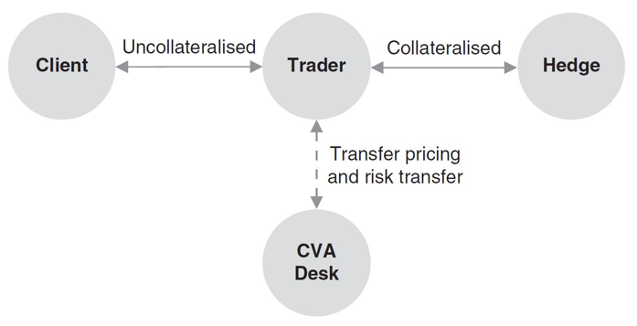
The hedges are usually collateralized (often even cleared) so most CVA comes from the initial transaction with the end client.

Summary of CVA usage

The CVA is used for:

• CCR-adjusted pricing and accounting:
  • CVA is charged to the client;
  • It must be reflected in derivatives valuation for accounting (IFRS 13);
• Trading decisions and CCR-adjusted performance attribution:
  • CVA is taken into account in trading decisions;
  • It is used for CCR-adjusted performance attribution for trading desks and divisions;
  • encouraging trades that diversify or reduce CCR.

CVA sensitivities are also computed and can be used for:

• CVA PnL prediction:
  • The CVA PnL can be approximated using Taylor expansion.
• Hedging:
  • CVA sensitivities are used to hedge the CVA by the CVA desk.
• CVA capital charge
  • During the GFC, CVA fluctuation led to more losses compared to defaults;
  • As a response, regulator now require a CVA capital charge for financial institutions;
  • It is a parametric value at risk on CVA based on CVA sensitivities.

Wrong Way Risk

In the CVA section, we stated that independence is assumed between the exposure and default. This is obviously not the case in reality, and correlation exists between them. It is called:

• Wrong Way Risk (WWR) when positive: default more likely when exposure is high, leading to higher CVA;
• Right Way Risk (RWR) when negative: default more likely when exposure is low, leading to lower CVA.

One can distinguish between two typs of WWR:

• General WWR, coming from macro-economic behavior, such as the dependance between default probabilites and general market risk-factors.
• Specific WWR, coming from the nature of the transactions with the counterparty.

For example, having an exposure that increases when oil price goes higher with EasyJet. or buying protection on a CDS on Société Générale from BNP Paribas. General WWR can be diversified to some extent, while specific WWR must be avoided.

Modelling WWR can be challenging. Various approaches exist, among which:

• Usage of stochastic default probabilities, correlated with the other risk factors.
• Jump approaches, where a jump in exposure is assumed to occur at counterparty default.
• Parametric approaches: linking the default probability with the exposure using a simple, parametric relationship.
• Stress testing and scenario analysis.

Challenges

Modelling challenge

As seen in previous sections, a multi-asset hybrid Monte-Carlo simulation is needed to accommodate the CCR and CVA computation requirements as:

• The exposure is not straightforward and depends on risk factors evolution;
• Market value grids on various dates and scenarios are needed;
• All transactions with the counterparty must be aggregated, in case of netting;
• In the presence of a CSA, collateral has to be simulated in the future.

Furthermore, the same Monte-Carlo simulation should be used to value all the trades:

• involving a global calibration (not product specific);
• diffusion of a high number of multi-asset correlated risk factors;
• pricing using closed-form formulae whenever possible.

The diffusion and pricing models have to be rich enough, but cannot be too sophisticated because of the computation burden as we will see next. So, usually, models with a small number of factors are favored. Furthermore, in terms of pricing methods, nested Monte Carlo or PDE cannot be afforded for exotics and American Monte-Carlo is usually used.

This difference in pricing models and methods between CCR/CVA and the base pricing done by each trading desk can lead to market value and exposure mismatches.

Computational challenge

The time consuming computation steps are the trades pricing and the aggregation. The calibration and diffusion cost is smaller as they are common to all trades, and done only once.

First, for the pricing, typical dimensions are:

• 10,000 Monte Carlo paths;
• 100 time steps (on average);
• 100 counterparts;
• 100 trades with each counterparty (on average).

Computing the MV grids requires 10 billion evaluations. Assuming each evaluation takes on average of 100 micro seconds, this means that 4H of computation time is needed on a 64core CPU to get the CVA figure. And an order of magnitude higher to get the CVA sensitivities… So, the tractability of the pricing models and the efficiency of the CCR / CVA pricing engine are key.

As for the aggregation, incremental CVA and PFE are needed in real-time or near real-time, for limits control on PFE, or to help make the trading decision for CVA. Here, the pricing involves one trade (or a few ones) so this step can be done relatively quickly, but the aggregation needs to be redone for the relevant netting set, including:

• update of the aggregate market value grid;
• simulation of the collateral balance;
• computation of the new exposure grid, then of the CVA, PFE, etc.

Continuous and rapid evolution

There has been a continuous stream of new regulations in the past years, aiming to reduce CCR in the wake of Lehman’s collapse.

A first example is the CVA capital charge, which is a VaR on CVA, requiring extra calculations. As a result, OTC derivatives consume more capital, that needs to be monitored, as this capital has a cost.

Another example is initial margin for OTC derivatives (cleared but also uncleared) which reduces CCR but implies high funding costs.

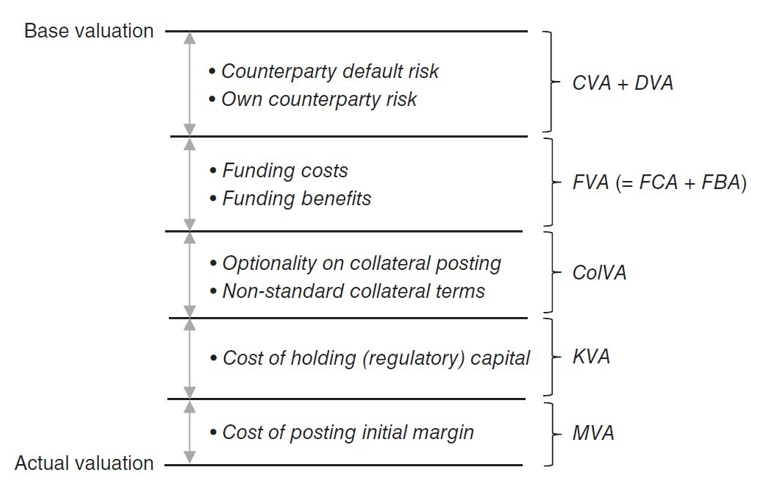
All of this leads to new XVA terms to take into account the total cost of the trade as illustrated bellow⁴:

• turning the CVA desk into an XVA desk
• and adding even more to the modelling and computational challenges.

Some of those additional XVA terms will be covered in future articles, so stay tuned!

References

1. BCBS-IOSCO, Margin Requirements for Non-Centrally Cleared Derivatives. 2015. ↩

2. For the latest version as of today: ISDA, ISDA SIMM methodology, version 2.4. 2021. ↩

3. See for example: Michael Pyhtin and Dan Rosen, Pricing Counterparty Risk at the Trade Level and CVA Allocations. 2011. ↩

4. Source: Jon Gregory, The XVA Challenge, 4th Edition. 2020. ↩ ↩²